An example of applying mSSA to the coefficients you created using pyEXP
This example assumes that you have run the Part1-Coefficients notebook to create the coefficients.
We begin by importing pyEXP and friends and setting the working directory.
[1]:
import os
import yaml
import math
import pyEXP
import numpy as np
import matplotlib.pyplot as plt

# In this test, I assume that you have already explored and run Part1-Coefficients. This notebook does some additional
# analysis and plotting
#
os.chdir('../Data')
Create the basis
This step is the same as in the previous notebook. We are going to use the basis for field evaluation so we need the basis.
[2]:
# Get the basis config
#
yaml_config = ""
with open('basis.yaml') as f:
    config = yaml.load(f, Loader=yaml.FullLoader)
    yaml_config = yaml.dump(config)

# Construct the basis instance
#
basis = pyEXP.basis.Basis.factory(yaml_config)
---- SLGridSph::ReadH5Cache: successfully read basis cache <sphereSL.model>
---- Spherical::orthoTest: worst=0.00016446
So far, this is the same as in Part1 … now:
Reading the halo coefficients
We created the halo coefficients in the last notebook and stashed them in the EXP HDF5 format. Now, we’ll read them back.
[3]:
# Reread the coefs from the file
#
coefs = pyEXP.coefs.Coefs.factory('test_coefs')

print("Got coefs for name=", coefs.getName())
Got coefs for name= dark halo
Visualizing the fields
We made a few test grids in Part 1 of the notebook. This time, we’ll make surface renderings:
[4]:
# Now try some slices for rendering
#
times = coefs.Times()
pmin = [-0.05, -0.05, 0.0]
pmax = [ 0.05, 0.05, 0.0]
grid = [ 40, 40, 0]
fields = pyEXP.field.FieldGenerator(times, pmin, pmax, grid)
surfaces = fields.slices(basis, coefs)
print("We now have the following [time field] pairs")
final = 0.0
for v in surfaces:
print('-'*40)
for u in surfaces[v]:
print("{:8.4f} {}".format(v, u))
final = v
# Print the potential image at the final time (I think there is a
# fencepost issue in this grid, no matter).
x = np.linspace(pmin[0], pmax[0], grid[0])
y = np.linspace(pmin[1], pmax[1], grid[1])
xv, yv = np.meshgrid(x, y)
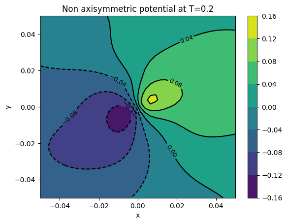
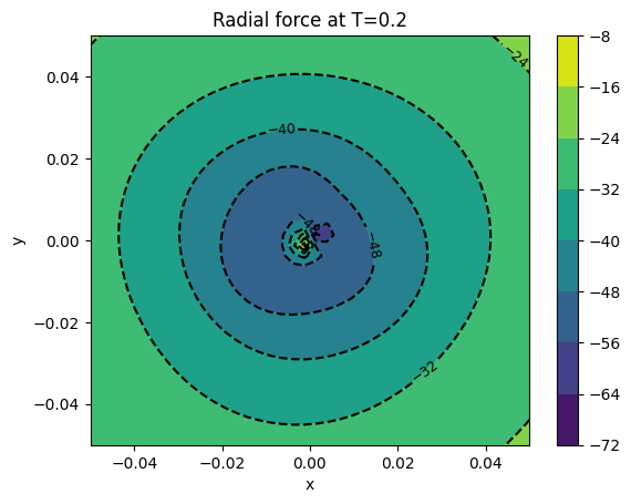
# Visualize the final time slice in grid. Obviously, we could use any
# field we want. Here is potential and radial force.
cont1 = plt.contour(xv, yv, surfaces[final]['potl m>0'], colors='k')
plt.clabel(cont1, fontsize=9, inline=True)
cont2 = plt.contourf(xv, yv, surfaces[final]['potl m>0'])
plt.colorbar(cont2)
plt.xlabel('x')
plt.ylabel('y')
plt.title('Non axisymmetric potential at T={}'.format(final))
plt.show()
cont1 = plt.contour(xv, yv, surfaces[final]['rad force'], colors='k')
plt.clabel(cont1, fontsize=9, inline=True)
cont2 = plt.contourf(xv, yv, surfaces[final]['rad force'])
plt.colorbar(cont2)
plt.xlabel('x')
plt.ylabel('y')
plt.title('Radial force at T={}'.format(final))
plt.show()
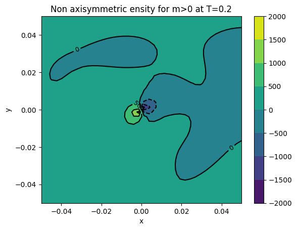
cont1 = plt.contour(xv, yv, surfaces[final]['dens m>0'], colors='k')
plt.clabel(cont1, fontsize=9, inline=True)
cont2 = plt.contourf(xv, yv, surfaces[final]['dens m>0'])
plt.colorbar(cont2)
plt.xlabel('x')
plt.ylabel('y')
plt.title('Non axisymmetric ensity for m>0 at T={}'.format(final))
plt.show()
We now have the following [time field] pairs
----------------------------------------
  0.0100  azi force
  0.0100  dens
  0.0100  dens m=0
  0.0100  dens m>0
  0.0100  mer force
  0.0100  potl
  0.0100  potl m=0
  0.0100  potl m>0
  0.0100  rad force
----------------------------------------
  0.0200  azi force
  0.0200  dens
  0.0200  dens m=0
  0.0200  dens m>0
  0.0200  mer force
  0.0200  potl
  0.0200  potl m=0
  0.0200  potl m>0
  0.0200  rad force
----------------------------------------
  0.0300  azi force
  0.0300  dens
  0.0300  dens m=0
  0.0300  dens m>0
  0.0300  mer force
  0.0300  potl
  0.0300  potl m=0
  0.0300  potl m>0
  0.0300  rad force
----------------------------------------
  0.0400  azi force
  0.0400  dens
  0.0400  dens m=0
  0.0400  dens m>0
  0.0400  mer force
  0.0400  potl
  0.0400  potl m=0
  0.0400  potl m>0
  0.0400  rad force
----------------------------------------
  0.0500  azi force
  0.0500  dens
  0.0500  dens m=0
  0.0500  dens m>0
  0.0500  mer force
  0.0500  potl
  0.0500  potl m=0
  0.0500  potl m>0
  0.0500  rad force
----------------------------------------
  0.0600  azi force
  0.0600  dens
  0.0600  dens m=0
  0.0600  dens m>0
  0.0600  mer force
  0.0600  potl
  0.0600  potl m=0
  0.0600  potl m>0
  0.0600  rad force
----------------------------------------
  0.0700  azi force
  0.0700  dens
  0.0700  dens m=0
  0.0700  dens m>0
  0.0700  mer force
  0.0700  potl
  0.0700  potl m=0
  0.0700  potl m>0
  0.0700  rad force
----------------------------------------
  0.0800  azi force
  0.0800  dens
  0.0800  dens m=0
  0.0800  dens m>0
  0.0800  mer force
  0.0800  potl
  0.0800  potl m=0
  0.0800  potl m>0
  0.0800  rad force
----------------------------------------
  0.0900  azi force
  0.0900  dens
  0.0900  dens m=0
  0.0900  dens m>0
  0.0900  mer force
  0.0900  potl
  0.0900  potl m=0
  0.0900  potl m>0
  0.0900  rad force
----------------------------------------
  0.1000  azi force
  0.1000  dens
  0.1000  dens m=0
  0.1000  dens m>0
  0.1000  mer force
  0.1000  potl
  0.1000  potl m=0
  0.1000  potl m>0
  0.1000  rad force
----------------------------------------
  0.1100  azi force
  0.1100  dens
  0.1100  dens m=0
  0.1100  dens m>0
  0.1100  mer force
  0.1100  potl
  0.1100  potl m=0
  0.1100  potl m>0
  0.1100  rad force
----------------------------------------
  0.1200  azi force
  0.1200  dens
  0.1200  dens m=0
  0.1200  dens m>0
  0.1200  mer force
  0.1200  potl
  0.1200  potl m=0
  0.1200  potl m>0
  0.1200  rad force
----------------------------------------
  0.1300  azi force
  0.1300  dens
  0.1300  dens m=0
  0.1300  dens m>0
  0.1300  mer force
  0.1300  potl
  0.1300  potl m=0
  0.1300  potl m>0
  0.1300  rad force
----------------------------------------
  0.1400  azi force
  0.1400  dens
  0.1400  dens m=0
  0.1400  dens m>0
  0.1400  mer force
  0.1400  potl
  0.1400  potl m=0
  0.1400  potl m>0
  0.1400  rad force
----------------------------------------
  0.1500  azi force
  0.1500  dens
  0.1500  dens m=0
  0.1500  dens m>0
  0.1500  mer force
  0.1500  potl
  0.1500  potl m=0
  0.1500  potl m>0
  0.1500  rad force
----------------------------------------
  0.1600  azi force
  0.1600  dens
  0.1600  dens m=0
  0.1600  dens m>0
  0.1600  mer force
  0.1600  potl
  0.1600  potl m=0
  0.1600  potl m>0
  0.1600  rad force
----------------------------------------
  0.1700  azi force
  0.1700  dens
  0.1700  dens m=0
  0.1700  dens m>0
  0.1700  mer force
  0.1700  potl
  0.1700  potl m=0
  0.1700  potl m>0
  0.1700  rad force
----------------------------------------
  0.1800  azi force
  0.1800  dens
  0.1800  dens m=0
  0.1800  dens m>0
  0.1800  mer force
  0.1800  potl
  0.1800  potl m=0
  0.1800  potl m>0
  0.1800  rad force
----------------------------------------
  0.1900  azi force
  0.1900  dens
  0.1900  dens m=0
  0.1900  dens m>0
  0.1900  mer force
  0.1900  potl
  0.1900  potl m=0
  0.1900  potl m>0
  0.1900  rad force
----------------------------------------
  0.2000  azi force
  0.2000  dens
  0.2000  dens m=0
  0.2000  dens m>0
  0.2000  mer force
  0.2000  potl
  0.2000  potl m=0
  0.2000  potl m>0
  0.2000  rad force
Using a point mesh instead of a grid
The FieldGenerator allows you to specify an array of Cartesian points for field evaluation. This way, you can get creative with geometries and mesh spacing. As an illustration, let us repeat the same renderings using this mesh-point method.
As a sanity check, let’s do the same plots as the grid example above.
[5]:
# First, we generate a Cartesian mesh
xy = np.linspace(-1, 1, 40)
mesh = np.ndarray((40*40, 3))
for i in range(40):
    for j in range(40):
        mesh[i*40+j, 0] = xy[i]
        mesh[i*40+j, 1] = xy[j]
        mesh[i*40+j, 2] = 0.0
Now that we have the a point set, in a Cartesian grid for this test, generate the points:
[6]:
fields = pyEXP.field.FieldGenerator(times, mesh)
points = fields.points(basis, coefs)
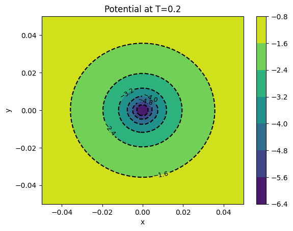
# Print the potential image at the final time (I think there is a
# fencepost issue in this grid, no matter).
x = np.linspace(pmin[0], pmax[0], grid[0])
y = np.linspace(pmin[1], pmax[1], grid[1])
xv, yv = np.meshgrid(x, y)
def tomesh(points):
ret = np.zeros(xv.shape)
print(ret.shape)
for i in range(40):
for j in range(40):
ret[i, j] = points[i*40+j]
return ret
# Visualize the final time slice in grid. Obviously, we could use any
# field we want. Here is potential and radial force.
img = tomesh(points[final]['potl'])
cont1 = plt.contour(xv, yv, img, colors='k')
plt.clabel(cont1, fontsize=9, inline=True)
cont2 = plt.contourf(xv, yv, img)
plt.colorbar(cont2)
plt.xlabel('x')
plt.ylabel('y')
plt.title('Potential at T={}'.format(final))
plt.show()
img = tomesh(points[final]['rad force'])
cont1 = plt.contour(xv, yv, img, colors='k')
plt.clabel(cont1, fontsize=9, inline=True)
cont2 = plt.contourf(xv, yv, img)
plt.colorbar(cont2)
plt.xlabel('x')
plt.ylabel('y')
plt.title('Radial force at T={}'.format(final))
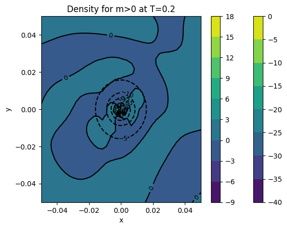
img = tomesh(points[final]['dens m>0'])
cont1 = plt.contour(xv, yv, img, colors='k')
plt.clabel(cont1, fontsize=9, inline=True)
cont2 = plt.contourf(xv, yv, img)
plt.colorbar(cont2)
plt.xlabel('x')
plt.ylabel('y')
plt.title('Density for m>0 at T={}'.format(final))
(40, 40)
(40, 40)
(40, 40)
[6]:
Text(0.5, 1.0, 'Density for m>0 at T=0.2')
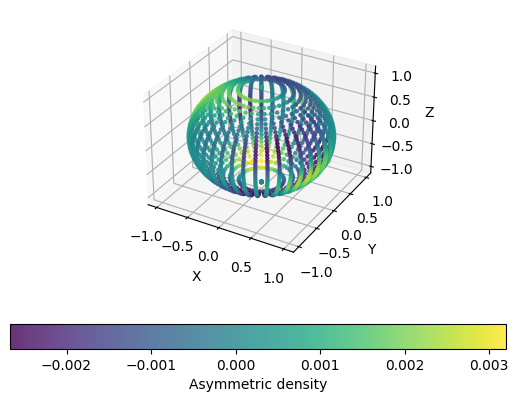
Now, let’s take advantage of the unstructured point set for something different
First, let’s make a point set on a spherical surface:
[7]:
# First, we generate a Cartesian mesh
phi  = np.linspace(0.0, 2.0*math.pi, 40)
cost = np.linspace(-1.0, 1.0, 40)
mesh = np.ndarray((40*40, 3))
radius = 1.0
for i in range(40):
    for j in range(40):
        sint = np.sqrt(1.0 - cost[j]**2)
        mesh[i*40+j, 0] = radius*sint*math.cos(phi[i])
        mesh[i*40+j, 1] = radius*sint*math.sin(phi[i])
        mesh[i*40+j, 2] = radius*cost[j]
Generate a new point set for this unstructured grid as follows:
[8]:
fields = pyEXP.field.FieldGenerator(times, mesh)
points = fields.points(basis, coefs)
Now, let’s make a 3d scatter plot with points colored by field values:
[9]:
fig = plt.figure()
ax = fig.add_subplot(projection='3d')

sc = ax.scatter(mesh[:,0], mesh[:,1], mesh[:,2], c=points[times[-1]]['dens m>0'], marker='o', s=5, alpha=0.8)

ax.set_xlabel('X')
ax.set_ylabel('Y')
ax.set_zlabel('Z')

plt.colorbar(sc, label='Asymmetric density', orientation='horizontal')
plt.show()
Using MSSA
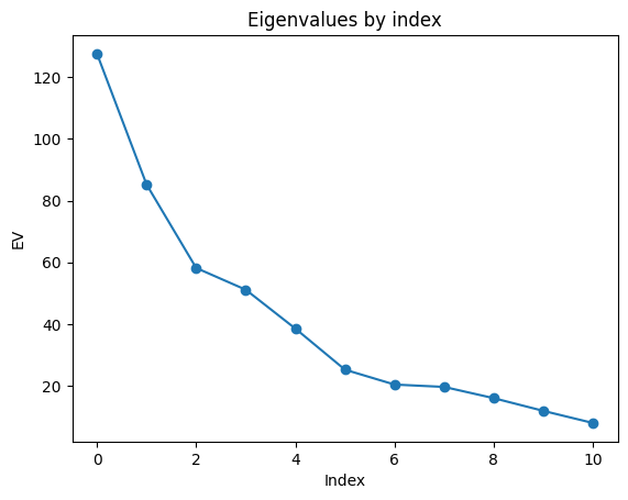
Generate the initial MSSA analyis and plot the run of eigenvalues
[10]:
# Make a subkey sequence
#
keylst = coefs.makeKeys([2])
print("Keys=", keylst)

name = 'dark halo'
config = {name: (coefs, keylst, [])}

# This is the window length.  The largest meaningful length is half
# the size of the time series.  We'll choose that here but it *is*
# interesting to retry these analyses with different window lengths.

window = int(len(coefs.Times())/2)
npc = 10

print("Window={} PC number={}".format(window, npc))

ssa = pyEXP.mssa.expMSSA(config, window, npc)

ev = ssa.eigenvalues()

plt.plot(ev, 'o-')
plt.xlabel("Index")
plt.ylabel("EV")
plt.title("Eigenvalues by index")
plt.show()
Keys= [[2, 0, 0], [2, 0, 1], [2, 0, 2], [2, 0, 3], [2, 0, 4], [2, 0, 5], [2, 0, 6], [2, 0, 7], [2, 0, 8], [2, 0, 9], [2, 1, 0], [2, 1, 1], [2, 1, 2], [2, 1, 3], [2, 1, 4], [2, 1, 5], [2, 1, 6], [2, 1, 7], [2, 1, 8], [2, 1, 9], [2, 2, 0], [2, 2, 1], [2, 2, 2], [2, 2, 3], [2, 2, 4], [2, 2, 5], [2, 2, 6], [2, 2, 7], [2, 2, 8], [2, 2, 9]]
Window=10 PC number=10
---- Eigen is using 4 threads
shape U = 500 x 11
shape Y = 11 x 500
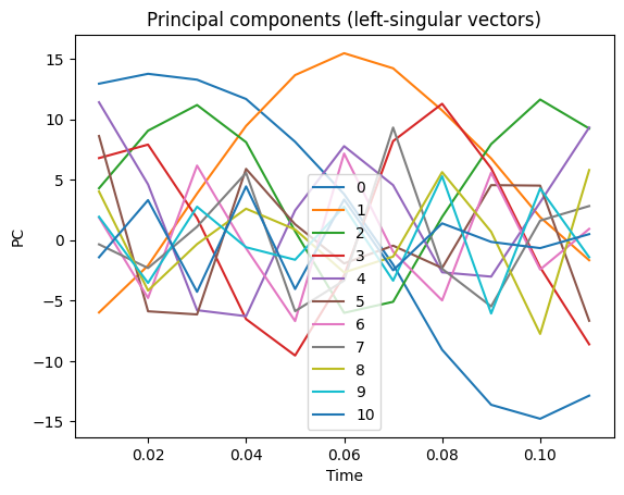
Next plot the principle components.
[11]:
times = coefs.Times();
pc    = ssa.getPC();

rows, cols = pc.shape

for i in range(cols):
    plt.plot(times[0:rows], pc[:,i], '-', label="{:d}".format(i))

plt.xlabel('Time')
plt.ylabel('PC')
plt.legend()
plt.title("Principal components (left-singular vectors)")
plt.show()
Now try a reconstruction
[12]:
coefs.zerodata() # <---replace with reconstructed
ssa.reconstruct([0, 1, 2, 3, 4, 5, 6, 7, 8, 9])
newdata = ssa.getReconstructed()
print('newdata is a', type(newdata))
newdata is a <class 'dict'>
Compute the k-means analysis
The k-means partitions n vector observations into k clusters in which each observation belongs to the cluster with the nearest centers while minimizing the variance within each cluster. In this case, the vectors are the full trajectory matrices and the distance is the distance between the trajectory matricies reconstructed from each eigentriple from mSSA. The distance used here is the Frobenius distance or matrix norm distance: the square root of the sum of squares of all elements in the difference between two matrices.
Note: the k-means analysis will use the reconstructions from your last call to reconstruct. In this notebook, that would be from the previous cell; the first 10 PCs. The k-means initial cluster selection chooses every second PC by default. This is a good choice for time series representing quasi-periodic motion which generally have pairs of PCs representing the sinusoidal behavior.
The k-means analysis illustrates the clear patterns in the PCs seen in the plots above: the individual features occur in pairs, dominated by the first two pairs as seen in the eigenvalue plot. This dominant pair is assigned id=0. The next pair is assigned id=1. The rest of the PCs are not particularly correlated and are lumped into id=0.
[13]:
# Print k-means groups, allowing up to 6
#
id, dist, tol = ssa.kmeans(clusters=6)

# Print the results
print('{:<4s} | {:<4s} | {:<13s}'.format('PC', 'id', 'distance'))
print('{:<4s} | {:<4s} | {:<13s}'.format('----', '----', '--------'))
for k in range(len(id)):
    print('{:<4d} | {:<4d} | {:<13.6e}'.format(k, id[k], dist[k]))
PC   | id   | distance
---- | ---- | --------
0    | 0    | 6.243771e+00
1    | 0    | 6.243771e+00
2    | 1    | 4.312612e+00
3    | 1    | 4.312612e+00
4    | 2    | 0.000000e+00
5    | 3    | 2.561358e+00
6    | 3    | 2.561358e+00
7    | 4    | 2.330193e+00
8    | 4    | 2.342835e+00
9    | 4    | 2.861371e+00
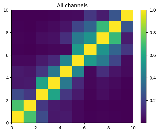
In this case, k-means identifies 5 groups: 3 pairs and triple. Compare this with the results from the w-correlation matrix in the next section…
You can see from the PCs themselves, that very few dynamical periods are available for analysis. This simulation is not long enough for a highly signficant cluster analysis.
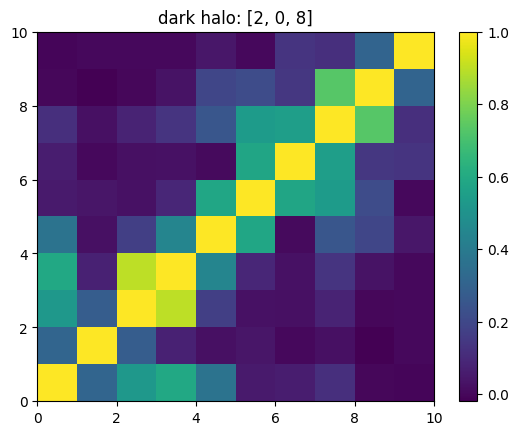
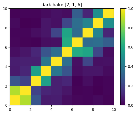
Finally plot the w-correlation matrix
This is the sum of the w-correlation matrices for all channels.
[14]:
mat = ssa.wCorrAll()
x = plt.pcolormesh(mat)
plt.title("All channels")
plt.colorbar(x)
plt.show()
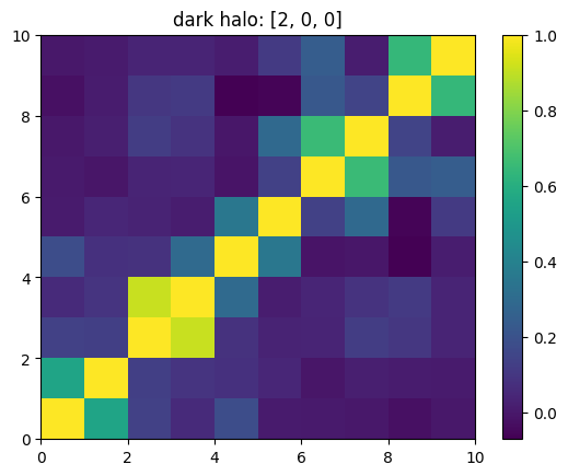
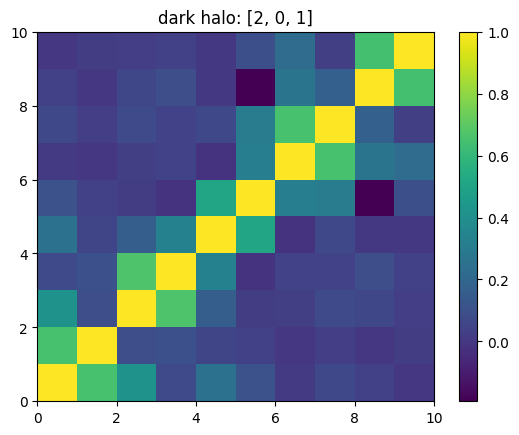
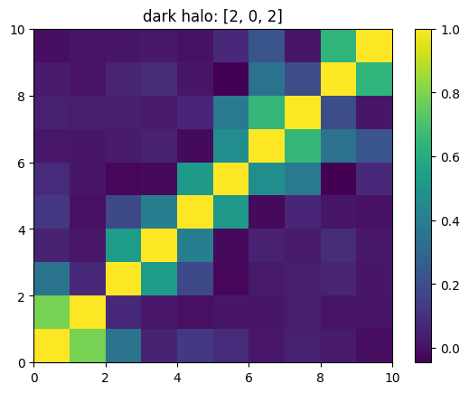
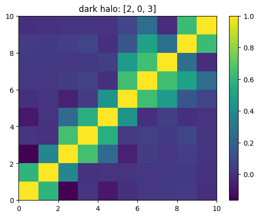
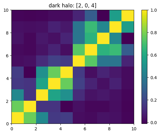
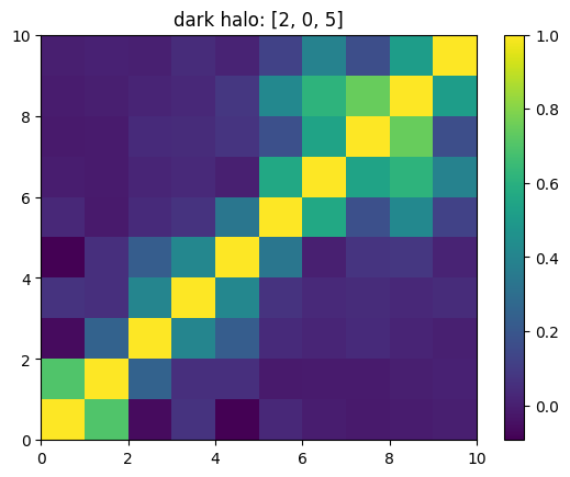
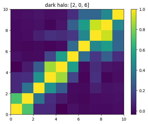
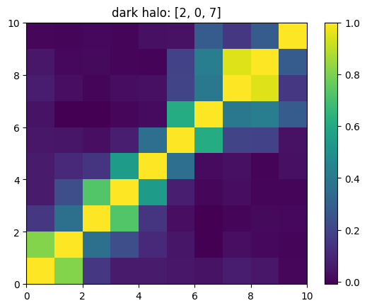
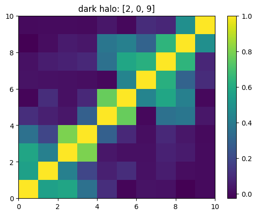
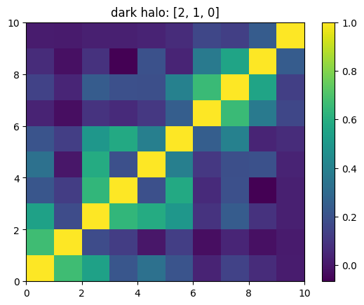
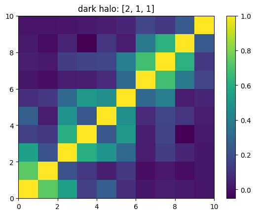
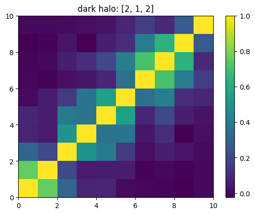
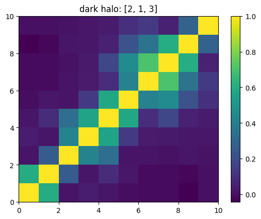
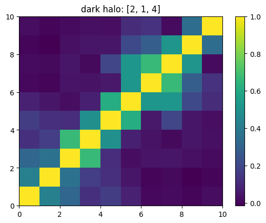
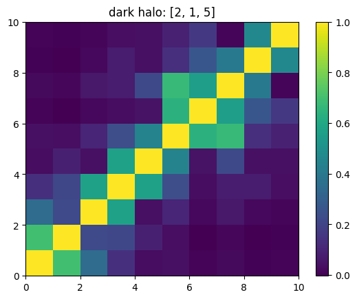
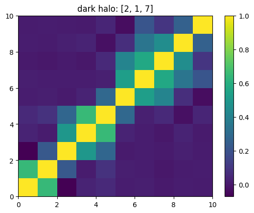
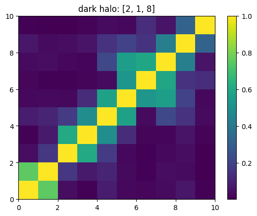
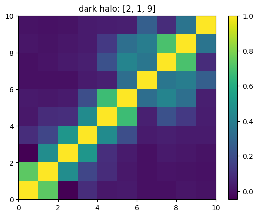
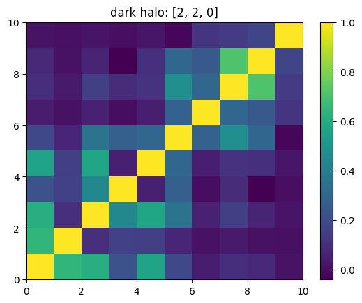
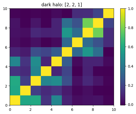
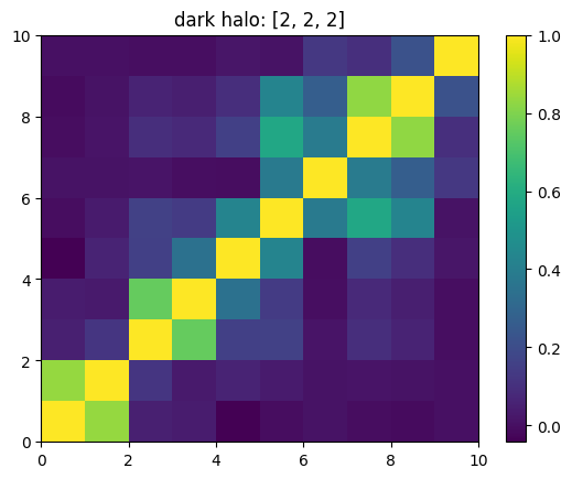
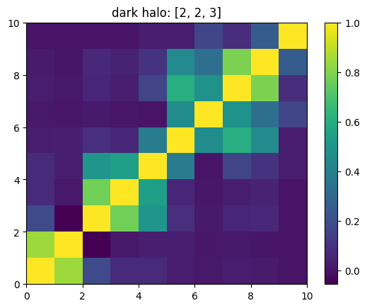
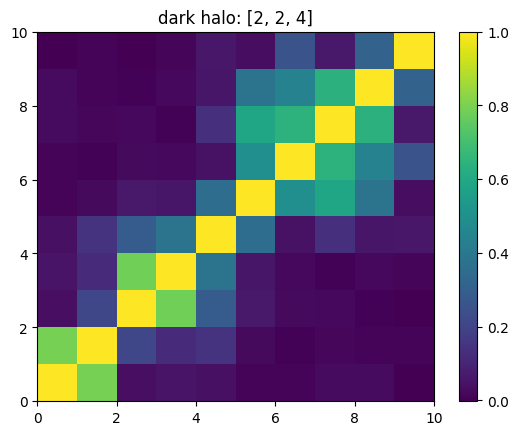
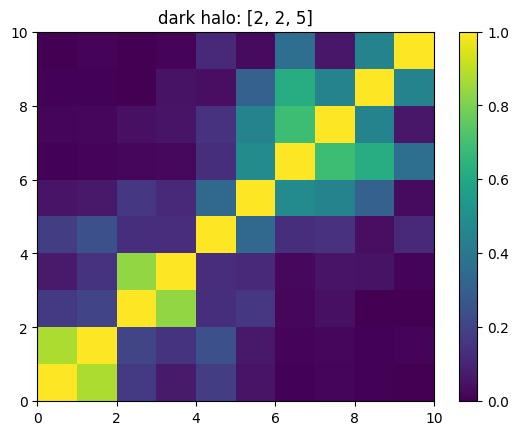
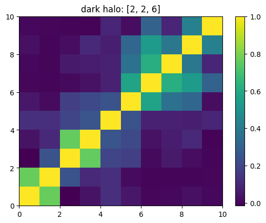
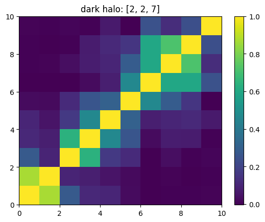
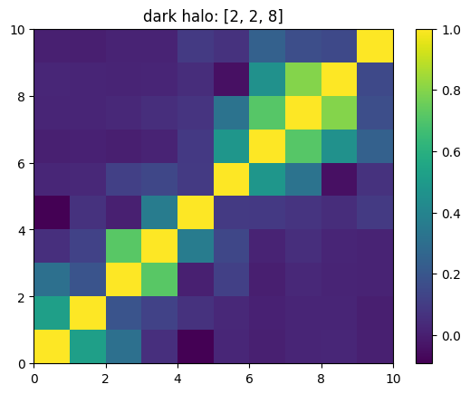
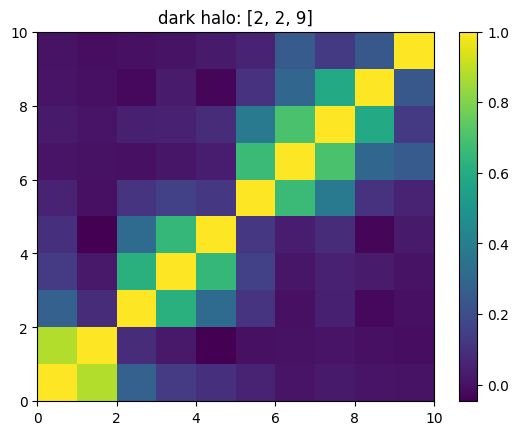
One can also look at individual channels.
[15]:
# Get and view the w-correlation matrices
# for each key individually
#
for k in keylst:
    mat = ssa.wCorr(name, k)
    # Plot it
    x = plt.pcolormesh(mat)
    plt.title('{}: {}'.format(name,k))
    plt.colorbar(x)
    plt.show()