BFE theory
The BFE method has four primary advantages over tree- and grid-method gravity solvers: (1) the computational effort in the force calculation scales linearly with particle number; (2) the dynamic range of multi-scale systems, such as the disk-halo system, can be better resolved by tailoring the geometry and scale of the density and potential variation to each of the components individually; (3) sensitivity to weak global distortions is possible because small-scale noise can be removed; and (4) intercomponent interactions can be explicitly selected and controlled to allow the study of different mechanisms individually. In particular, EXP is designed to allow the self-gravity and intercomponent forces between all components to be independently selected and controlled by simple configuration parameters (see What is YAML?).
In the remainder of this chapter, I will give a brief introduction to the mathematics of the BFE method which then motivates the overall software design. This should provide enough review of the background to begin using the code (EXP tutorial and pyEXP tutorial). Additional technical details will be summarized in later chapters.
The basic BFE algorithm
The harmonic basis-function expansion (BFE) technique has been used to both study and compare simulations to theoretical predictions, owing to its natural relationship with analytic perturbation theory ([weinberg07a], [weinberg07b]}. To use the BFE approach for n-body simulations, one uses the biorthogonal nature of the appropriately chosen basis functions to solve the Poisson equation using separable azimuthal harmonics at the same time as the expansion. A biorthogonal system is a pair of indexed families of vectors in some topological vector space such that the inner product of the pair is the Kronecker delta. The BFE method constructs a biorthongal system \(d_j(\mathbf{x}), p_k(\mathbf{c})\) such that \(\nabla^2 p_i = 4\pi G d_i\) and \(\int d\mathbf{x}\, d_j(\mathbf{x}) p_k(\mathbf{x}) = 4\pi G\delta_{jk}.\) Let the density of our particle distribution of \(N\) points with masses \(m_i\) described by
Then, approximations for the density and potential fields are
where
Generally, any technique making use of these properties may be called BFE ([cluttonbrock72], [cluttonbrock73], [kalnajs76], [hernquist92], [earn96], [weinberg99]). BFE has many notable features that make them ideal for studying disturbances to equilibrium stellar discs. For simulations using BFE methods, harmonic function analysis decomposes a distribution into linearly-summable functions that resemble expected evolutionary scenarios in disc galaxy evolution. The primary diagnostics available are the amplitude and phase of each function. In addition, the time-dependence of the coefficients themselves provides another dimension for studying evolution that may not clearly manifest itself in analytic studies (see mSSA and [weinberg21]). Using harmonic function analysis in BFE simulations – no matter what Poisson solver – is reconstruction of the potential at any time in the simulation, for any arbitrary combinations of particles.
Empirical Orthogonal Functions
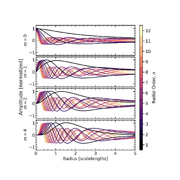
Fig. 1 In-plane amplitude variations as a function of disk scale length for all radial functions per harmonic order in the cylindrical disk basis. We show the \(m=0,1,2,4\) harmonic subspaces as panels from top to bottom. The amplitude in each panel has been normalized to the maximum in the corresponding subspace. Functions that are zero everywhere are vertically asymmetric.
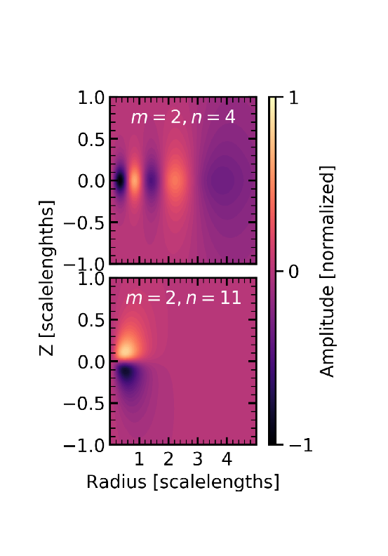
Fig. 2 Examples of vertically symmetric (\(m=2,n=4\), upper panel), and vertically asymmetric (\(m=2,n=11\), lower panel) functions for the disk basis. The \(x\) and \(z\) axis correspond to the radial and vertical axes in the simulation, and the amplitude of the variations between panels has been normalized to the maximum \(m=2\) amplitude.
A BFE computes the gravitational potential by projecting particles onto a set of biorthogonal basis functions that satisfy the Poisson equation as described in [petersen2022]. Then, the force at the position of each particle is evaluated from the basis-function approximation to the field at the particle position. Fundamentally, this approach relies on the mathematical properties of the Sturm-Louiville equation (SLE) of which the Poisson equation is a special case. The SLE describes many physical systems, and may be written as:
where \(\lambda\) is a constant, and \(\omega(x)\) is a weighting function. The eigenfunctions \(\phi_j\) of the SLE form a complete basis set with eigenvalues \(\lambda_j\), where \(j\) may be truncated from the theoretically infinite series. When applied to the Poisson equation specifically, the equation separates in conic coordinate systems. For Cartesian, the widely-used Fourier expansion is a well-known examples. The BFE potential solver is built using properties of eigenfunctions and eigenvalues of the SLE.
For an expansion in spherical harmonics, the SLE/Poisson equation separates into angular and radial equations, giving rise to spherical harmonics and Bessel functions naturally. The boundary conditions are easy to apply in radius (at the origin and at infinity). For example, a dark-matter halo can be expanded into a relatively small number of spherical harmonics \(Y_{lm}\) and appropriate radial functions. Each term in halo potential is given by \(\Phi_{lm}^j = \phi_{lm}^j(r)Y_{lm}(\theta,\phi)\). Even more interesting, Bessel functions are not the only choice. By changing the weighting function we may derive an infinity of radial bases. In particular, the weighting function \(\omega\) in equation (1) may be selected to be an equilibrium solution of the Poisson equation. In other words, the unperturbed potential would be represented by a single term!
The disk is more complicated. Although one can construct a disk basis from the eigenfunctions of the Laplacian as in the spherical case (e.g. [earn96]), the boundary conditions in cylindrical coordinates make the basis hard to implement. To get around this, our solution method starts with a spherical basis with \(l\le36\) and uses a singular value decomposition (SVD) to define a rotation in function space to best represent a target disk density. Specifically, each density element \(\rho(R, z)\,d^3x\) contributes
to the expansion coefficient \(a_{lm}^j\), or
where \(R, z\) are the radial and vertical cylindrical coordinates. The second equation shows the approximation for \(N\) particles where \(\sum_i m_i = \int \rho(R, z)d^3x\).
The covariance of the coefficient given the density \(\rho(R, z)\), \(\mbox{cov}(\mathbf{a})\), is constructed similarly. For each azimuthal harmonic \(m\), all spherical terms \(l\ge m\) and radial indices \(j\) are covariant. So the full matrix may be separated into blocks for each \(m\). Each block in the covariance matrix describes which terms \(a_{lm}^j\) contribute the most variance for a particular \(m\). By diagonalizing \(\mbox{cov}(\mathbf{a}),\) we may find a new basis, uncorrelated by the target density. Because \(\mbox{cov}(\mathbf{a})\) is symmetric and positive definite, all eigenvalues will be positive. The term with the largest eigenvalue describes the majority of the correlated contribution, and so on for the second largest eigenvalue, etc. EXP performs this diagonalization using the singular value decomposition (SVD) and the singular matrices (now mutual transposes owing to symmetry) describe a rotation of the original basis into the uncorrelated basis.
The new basis functions optimally approximate the true distribution from the spherical-harmonic expansion in the original basis in the sense that the lagest amount of variance is contained in the smallest number of terms; we might call this optimal in the least-squares sense. Since the transformation and the Poisson equation are linear, the new eigenfunctions are also biorthogonal. The new coefficient vector is related to the original coefficient vector by an orthogonal transformation. Because we are free to break up the spherical basis into meriodinal subspaces by azimuthal order, the resulting two-dimensional eigenfunctions in \(r\) and \(\theta\) are equivalent to a decomposition in cylindrical coordinates \(r,~z,\) and \(\theta\). We condition the initial disk basis functions on an analytic disk density such that the lowest-order potential-density pair matches the initial analytic mass distribution. This choice also acts to reduce small-scale discreteness noise as compared to conditioning the basis function on the realized positions of the particles [weinberg98]. Although there could be some other biases introduced by this procedure, our experience to date suggests that this approach provides a fair representation of the disk density and potential fields.
We can represent the potential and density of a galaxy as a superposition of several basis functions. This allows us to decompose the galaxy based on its geometry and symmetry. For an initially axisymmetric example, azimuthal harmonics \(m\), where \(m=0\) is the monopole, \(m=1\) is the dipole, \(m=2\) is the quadrupole, and so on, will efficiently summarize the degree and nature of the asymmetries. The sine and cosine terms of each azimuthal order give the phase angle of the harmonic that can be used to calculate the pattern speed. For disks, each azimuthal harmonic represents both the radial and vertical structure simultaneously; that is each basis function is a two-dimensional meridional plane multipled by \(e^{im\phi}\). The symmetry of the input basis and the covariance matrix further demands that the singular value decomposition produce vertically symmetric or anti-symmetric functions. See Visualizing bases for examples of both types of functions and hints on how to explore them using pyEXP.
After some exploration, we determined that a radial scale factor for the spherical profile of approximately \(\sqrt{2}\) time larger than spherical deprojected profile of the disk represented the disk profile is the smallest number of terms. This choice of radial scale is not very sensitive to the resulting basis, however.
Examples
Fig. 1 shows the in-plane amplitude variations for radial functions (\(n\) orders) as a function of radius, separated by harmonic subspace (\(m\) orders) for an exponential disk in an NFW ([navarro97]) halo. We show the four harmonic subspaces that are most relevant for the evolution of the simulation, \(m=0,1,2,4\), from top to bottom in the panels. In each harmonic subspace, the lowest-order radial order, \(n=1\), has no nodes except at \(R=0\) for \(m\ge0\). The number of nodes increases with order \(n\). The nodes are interleaved by radial order, but the increasing number of nodes means that the smallest radius node always decreases in radius as the number of nodes increases. Therefore, an increase in amplitude for higher–\(n\)–order harmonics corresponds to the movement of mass to smaller radii. Additionally, the spacing of nodes gives an approximate value for the force resolution of the simulation. For example, the highest order \(m=0\) radial function (\(n=12\)) has a zero at \(R=0.2a\), or 600 pc in a MW-like galaxy, where \(a\) is the scale length. Additionally, the radial orders are interleaved between harmonic orders, such that the location of the first node, \(R^{[1st]}\), is given by
The lowest-order basis function exactly matches the initial density profile and has no nodes. In this example, the highest-order basis function, \(n=12\), would only imply a spatial resolution of 100 pc, the basis resolves a power law in density down to 10 pc. This choice removes or filters high spatial frequencies that may increase relaxation noise. Fig. 2 illustrates the vertical structure in the disk basis functions. The upper panel shows the \(m=2,n=4\) basis function in radius–z space. This function is symmetric about the \(z=0\) axis. The combination of vertically symmetric and asymmetric harmonics represent all possible variations in the gravitational field above and below the plane consistent with the spatial scales in the basis. In both panels, the color has been normalized to the maximum amplitude of the \(m=2\) harmonic subspace.
Two-dimensional cylindrical bases
The latest version of EXP includes support for two-dimensional cylindrical disk bases with three-dimensional potential theory. This allows full gravitational couples between two- and three-dimensional components.
Implementation
We construct two-dimensional polar bases using the same empirical orthogonal function (EOF) technique used to compute the three dimensional cylindrical basis (see empirical orthogonal functions). The user has the choice to two possible input basis:
The cylindrical Bessel functions of the first kind, \(J_m(\alpha_{m,n}R/R_{max})\) where \(\alpha_{m,n}\) is the nth root of \(J_m\) and \(R_{max}\) is an outer boundary. Thus, orthogonality is defined over a finite domain by construction.
The Clutton-Brock two-dimensional basis ([cluttonbrock72]) which orthogonal over the semi-infinite domain.
The user then chooses a conditioning density. Currently, these must be one of: exponential disk, Kuzmin (Toomre) disk, or Mestel disk ([bt08]). The code was written to allow for a user-defined density function and this will be implemented when needed in a future release.
The coupling between the two-dimensional disk and other three-dimensional components (e.g. the dark-matter halo or a bulge) requires evaluating the gravitational potential and its gradient everywhere in space. The three-dimensional gravitational potential is not automatically provided by the two-dimensional recursion relations that define the biorthogonal functions but must be evaluated by Hankel transform. This can be done very accurately over a finite domain with the quasi-discrete Hankel transformation on a finite domain (QDHT, [guizar04]). This algorithm exploits the special properties of the Bessel functions.
The EOF basis solutions are tabled on a fine grid and interpolated as needed. This is numerically efficient and accurate. While the in-plane density, potential and force fields are one-dimensional functions for each azimuthal order \(m\) and radial order \(n\), the potential and force fields for \(|z|>0\) require two-dimensional tables. Like the one-dimensional functions, these are finely-grided an interpolated using bilinear interpolation.
Discussion
The upside of the current strategy is:
One can condition the biorthgonal Bessel-function basis on any target density, similar to the three-dimensional case
The Hankel transform over the basis is very accurate so the whole thing is accurate.
The downsides are:
The Hankel transformation for an infinite domain is numerically challenging and we have had good success using QDHT, so we recommend the finite basis for this reason. This restriction to a finite-domain is not a problem in practice; all of the numerical implementations are finite.
The Bessels are wiggly and if one looks closely they leave their wiggly imprint at larger radii. Of course, we generally don’t care about larger radii.
While the code allows the conditioning on the 2d Clutton-Brock basis, the computation of the vertical potential is less accurate for the same computational work using QDHT. This could be improved by truncating the basis and implementing Neumann boundary conditions with appropriate outgoing eigenfunctions. That has not been done here. Another solution might be an asymptotic numerical evaluation of the Hankel transform at large cylindrical radii patched onto a brute force quadrature at small radii. At this point, we recommend the Bessel basis for accuracy if you need to couple to another three-dimensional component. If you only need the two-dimensional in-plane evaluations (e.g. a two-dimensional disk in a fixed halo), both basis choices will be good.
Three-dimensional rectangular bases
The latest version of EXP includes support for a three-dimensional rectangular prism using the classic trigonometric basis with periodic or reflective boundary conditions. This basis is ideal for investigating various aspects of gravitational kinetics or secular theory. There is no loss of generality in assuming that the prism is the unit cube and we will do that here. A rectangle prism with arbitrary lengths in each dimension can always be scaled to the unit cube.
The basis
Most will be familiar with the standard separation of the Poisson equation in Cartesian coordinates. Assume that the potential is
where \(\mathbf{k}=2\pi\mathbf{n}\) where \(\mathbf{n}\) is a triple of natural integers and \(C_{\mathbf{k}}\) is a normalization constant to be determined. Then:
This Sturm-Liouville equation has complete and orthogonal eigenfunctions – the trigonometric functions periodic in the unit cube – that we are using as our basis. The orthogonality condition demands that:
Assuming \(G=1\) implies that \(C_n = 1/\sqrt{2n^2}\).
We can think of this periodic cube as tiling all of space as a special case of the infinite homogeneous system. Therefore, the equilibrium has a constant density and constant potential. The constant (or DC) term \(\Phi_{0,0,0}\) exerts no force and does not consistently satisfy the Poisson equation (see [bt08] for more discussion of the so-called Jeans swindle).
Implementation
As described in The basic BFE algorithm, a particle ensemble immediately yields a set of coefficients: \(a_{\mathbf{n}}\). They take complex values but any physical quantity is real by construction. Numerically, the coefficients are accumulated by constructing the basis functions by recursion. For example, since
we only need the expensive evaluation of \(e^{i2\pi x}\), \(e^{i2\pi y}\), \(e^{i2\pi z}\) for each particle position \((x, y, z)\) and all the basis functions follow by successive multiplication.
Boundary conditions
Your particles only contribute to the density if they are inside the unit cube. Specifically, the Cube routine does not wrap the positions periodically into the unit cube. If you would like phase-space positions to be wrapped into the unit cube, use the PeriodicBC external routine with origin at zero, lengths of one, and periodic boundary conditions (these are the PeriodicBC defaults). The PeriodicBC allows periodic (‘p’), reflecting (‘r’), and vacuum (‘v’) boundary conditions. The boundary-condition-type parameters are passed as a string to the Cube routine with desired boundary conditions for ‘xyz’. For example, periodic boundary conditions in each dimension is ‘rrr’. Boundary condition type may be different in each axis.
Three-dimensional periodic slab bases
The latest version of EXP includes support for slab basis that is periodic in the unit square with equilibrium self-gravity in the vertical dimension. The coordinate system is Cartesian and Poisson equation separates in Cartesian coordinates. Since the equilibrium in the horizontal directions is uniform, the natural basis is trigonometric, e.g. \(e^{i2\pi (k_x x + k_y y)}\) where \(k_x, k_y\in\mathbb{Z}\). The resulting unknown basis functions satisfy
We assume an equilibrium solution \(d^2\Psi_o(z)/dz^2 = 4\pi G\rho_o(z)\) and write \(\Psi(z) = \Psi_o(z)u(z)\). Substituting this into the Poisson equation above and multiplying by \(\Psi_o(z)\), we obtain a Sturm-Liouville differential equation, eq. (1), with eigenfunctions \(u(z)\) and eigenvalues \(\lambda\) with
Implementation
The SLE is straightforwardly solved using the shooting algorithm in SLEDGE [pruess_fulton93]. The boundary conditions for the spherical solution are the natural ones for typical gravitational system at large radii. However, the potential and mass of our periodically-infinite slab is unbounded, rising linearly to infinity as \(|z|\rightarrow\infty\). Furthermore, our construction of the weighed SLE from the Poisson equation requires a non-zero weighing function \(\omega(z)\). We accomplish this by
Choosing a maximum vertical extent \(z_{max}\)
Evaluating the potential at some point outside this range, e.g. \(K\equiv\Psi_o(z_{max}[1+\delta])\)
Subtracting this value from the potential: \(\bar{\Psi}(z) = \Psi_o(z) - K\)
Adding a constant to the potential will not change the physical properties of the solution. A basis with different values of \(K\) will differ in scale but remain biorthogonal and valid solutions of the Poisson equation. The value of \(\delta>0\) is unimportant as long as \(\bar{\Psi}(z)\not=0\) in \(|z|\le z_{max}\). Finally, the SLE basis solutions are tabled on a fine grid and interpolated as needed. The horizontal, trigonometric part of basis is constructed by recursion as needed.
Usage notes
The user accessible parameters that may be specified in the YAML configuration (see the YAML config example) include:
nmaxx: the maximum number order in the x direction. These basis functions are periodic in x and have wave number \(n_x=-n_{x\,max}\) through \(n_x=n_{x\,max}\).
nmaxy: the maximum number order in the y direction.
nmaxz: the maximum number order in the z direction. These are basis functions will be index from 0 to nmaxz-1.
nminx: restrict the minimum wave number for x dimension to \(n_x\geq n_{x\,nmin}\)
nminy: restrict the minimum wave number for y dimension
hslab: scale height for slab basis
zmax: maximum height for slab basis
ngrid: number of grid points for basis table (default is 1000)
type: the base model for the slab. Choices are \(\rho(z)\propto\mbox{sech}^2(z/h), 1-(z/h)^2, \mbox{constant}\) which are denoted as isothermal, parabolic, and constant, respectively. The default is isothermal or (iso for short).
Final comments and caveats
The basic expansion algorithm is described at the beginning of this chapter. EXP can be configured to log coefficients at each step or in any multiple of steps (see Software design goals and features and What is YAML?). Additional details about using multiple time-step levels along with the leap-frog algorithm can be found in Section N-Body optimization in EXP. The coefficients for each \(n\) order are generally complex. The real and imaginary parts correspond to the cosine and sine components of the analogous Fourier terms \(A_m\) and \(B_m\). The coefficients are written in sine and cosine form for easy interpretation. Thus, the user may compute the phase angle for any basis function and use the total amplitude or modulus as an indicator of power.
The BFE approach trades off precision and degrees-of-freedom with adaptability. The truncated series of basis functions intentionally limits the possible degrees of freedom in the gravitational field in order to provide a low-noise, bandwidth-limited representation of the gravitational field. One must investigate whether the basis can capture all possible mechanisms of disk evolution. For example, this method will work very well for near equilibrium systems but could give biased results for grossly asymmetric systems. A simple example of this is centering (see Sec. EJ). Please be vigilant.
On the up side, a basis function representation provides an information–rich summary of the gravitational field and provides insight into the overall evolution. This method allows for the decomposition of different components into dynamically-relevant subcomponents for which the gravitational field can be calculated separately.
J. Binney and S. Tremaine. Galactic Dynamics: Second Edition. Princeton University Press, Princeton, NJ USA, 2008.
M. Clutton-Brock. The Gravitational Field of Flat Galaxies. APSS, 16:101–119, Apr. 1972.
M. Clutton-Brock. The Gravitational Field of Three Dimensional Galaxies. APSS, 23:55–69, July 1973.
D. J. D. Earn. Potential-Density Basis Sets for Galactic Disks. ApJ, 465:91, July 1996.
M. Guizar-Sicairos and J. C. Gutiérrez-Vega. Computation of quasi-discrete Hankel transforms of integer order for propagating optical wave fields. J. Opt. Soc. Am. A 21(1):53-58, 2004.
L. Hernquist and J. P. Ostriker. A self-consistent field method for galactic dynamics. ApJ, 386:375–397, Feb. 1992.
A. J. Kalnajs. Dynamics of Flat Galaxies. II. Biorthonormal Surface Density-Potential Pairs for Finite Disks. ApJ, 205:745–750, May 1976.
S.Pruess and C. T. Fulton. Mathematical software for Sturm-Liouville problems. ACM Trans. Math. Softw., 19:360-376, 1993.
Weinberg M. D. MNRAS, 297:101, June 1998.
Weinberg. AJ, 117:629, Jan. 1999.
M. D. Weinberg and N. Katz. The bar-halo interaction - I. From funda- mental dynamics to revised N-body requirements. MNRAS, 375:425–459, Feb. 2007
M. D. Weinberg and N. Katz. The bar-halo interaction - II. Secular evolution and the religion of N-body simulations. MNRAS, 375:460–476, Feb. 2007.
M. D. Weinberg and M. S. Petersen. Using multichannel singular spectrum analysis to study galaxy dynamics. MNRAS, 501:5408-5423, Mar. 2021
M. S. Petersen, M. D. Weinberg, and N. Katz. EXP: N-body integration using basis function expansions. MNRAS, 510:6201-6217, Mar. 2022