How to use mSSA with your coefficient series in pyEXP
There are a number of examples, tutorials, and how-to code and Jupyter notebooks for getting started with mSSA on the GitHub . Here we provide an example of running mSSA, plotting the eigenvalues and principal components (PCs), and reconstructing the bases.
Begin with the usual imports
import os
import copy
import yaml
import time
import pyEXP
import numpy as np
import matplotlib.pyplot as plt
from matplotlib import ticker
from os.path import exists

plt.rcParams['figure.figsize'] = [12, 9]
Switch to the working directory
I like to be explicit about my working directory but you don’t need to do this here. It would be sufficient to simply pass the full path to the coefficient factory below.
# os.chdir('/data/Nbody/Run101')
Read the EXP config files and generate the bases
# Read the basis info from the EXP file
#
exp_config = 'step3_try25.yml'
stride     = 2 #stride length
npc        = 40 #number of principal components (PCs)
size       = 0.05 #min/max of x, y axes for later plotting
npix       = 50 #number of pixels in grid for later plotting

# Open and read the EXP yaml file.  Get the runtag. Create the bases
# and construct coefficient file names
#
config = {}
basis  = {}
fcoef  = {}
runtag = ""

with open(exp_config, 'r') as f:
    yaml_db = yaml.load(f, Loader=yaml.FullLoader)

    # Get the runtag
    #
    runtag = yaml_db['Global']['runtag']
    print("\nRuntag from {} is: {}".format(exp_config, runtag))


    # Grab YAML force stanzas for all components
    #
    for v in yaml_db['Components']:
        comp = v['name']
        config[comp] = yaml.dump(v['force'])

        # Construct the basis instance
        #
        basis[comp] = pyEXP.basis.Basis.factory(config[comp])

        # Get the coefficient files
        fcoef[comp] = 'outcoef.{}.{}.h5'.format(comp, runtag)
        print("\nCoef file is:", fcoef[comp])
Runtag from step3_try25.yml is: run45_3

Coef file is: outcoef.dark.run45_3.h5
---- SLGridSph::write_cached_table: done!!
---- EmpCylSL::cache_grid: file read successfully
---- EmpCylSL::read_cache: table forwarded to all processes

Coef file is: outcoef.star.run45_3.h5
SLGridSph: opened <.slgrid_sph_cache>
Slave    0: tables allocated, MMAX=6
Read the coefficients and generate MSSA files
# Just do star component for now
#
comp = 'star'

coefs0 = pyEXP.coefs.Coefs.factory(fcoef[comp], stride=stride)
coefs  = coefs0.deepcopy()

# Make some custom [m, n] pairs
keylst = {}
for m in range(7):
    keylst[m] = coefs.makeKeys([m])


ssa = {}
ev  = {}
cum = {}

totPow = 0.0

for m in range(7):

    config = {coefs.getName(): (coefs, keylst[m], [])}

    window = int(len(coefs.Times())/2)
# Make some parameter flags as YAML.  The defaults should work fine
# for most people.
# totPow = True, detrend according to the total power
# noMean = True, do not subtract the mean when reading in channels
# (noMean = True is valid only for totPow detrending method)
# RedSym = True, use the randomized symmetric eigenvalue solver
# (RedSym) rather than RedSVD. This toggle is mainly for checking
# the accuracy of the default randomized matrix methods

    flags ="""
---
RedSym : true
# totPow : true
# noMean : true
...
"""
    print("Window={} PC number={}".format(window, npc))

    startTime = time.time()
    ssa[m] = pyEXP.mssa.expMSSA(config, window, npc, flags)
    file = '{}_{}_{}'.format(runtag, comp, m)
    if os.path.exists(file+"_mssa.h5"):
        ssa[m].restoreState(file)
    totPow += ssa[m].getTotPow()
    ev[m] = ssa[m].eigenvalues()
    cum[m] = ssa[m].cumulative()
    if not os.path.exists(file+"_mssa.h5"):
        ssa[m].saveState(file)
        print('Computed eigenvalues in {:6.2f} seconds'.format(time.time() - startTime))
Window=750 PC number=40
Window=750 PC number=40
Window=750 PC number=40
Window=750 PC number=40
Window=750 PC number=40
Window=750 PC number=40
Window=750 PC number=40
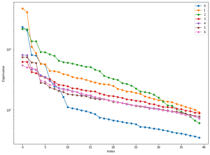
Plot the eigenvalues
# Make a plot of the eigenvalues
#
for m in range(7):
    plt.semilogy(ev[m], '-o', label=str(m))
plt.xlabel('Index')
plt.ylabel('Eigenvalue')
plt.legend()
plt.show()
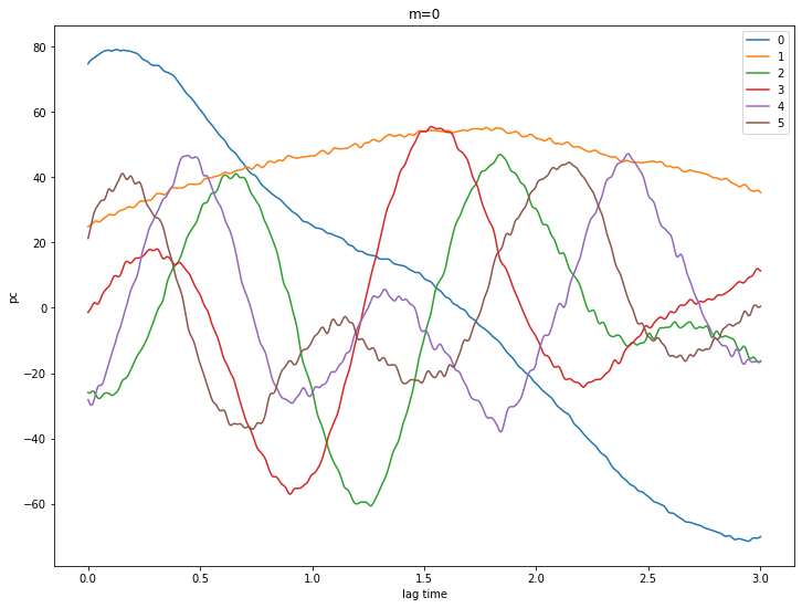
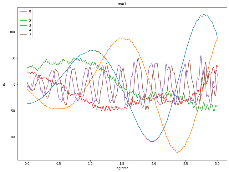
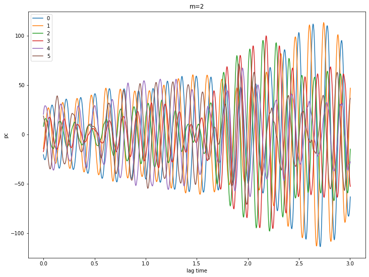
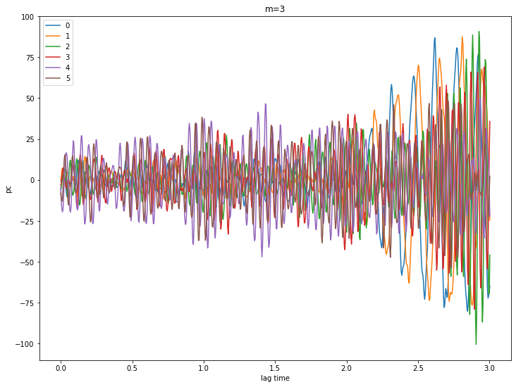
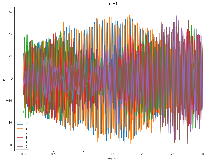
Let’s look at some PCs
for m in [0,1,2,3,4]:
    pcs = ssa[m].getPC()
    ntim = pcs.shape[0]
    for n in range(6):
        plt.plot(coefs.Times()[0:ntim], pcs[:,n], label=str(n))
    plt.xlabel('lag time')
    plt.ylabel('pc')
    plt.legend()
    plt.title('m={}'.format(m))
    plt.show()
# try a reconstruction using m = 2 and eigenvalues 0 - 3
ssa[2].reconstruct([0,1,2,3])
# zero all but the reconstructed
coefs.zerodata()
ssa[2].getReconstructed()
print(len(coefs.Times()))
1501
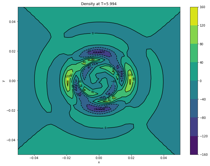
Check by making some surface renderings
Uses the final time slice but you could easily loop through all of them to make a movie, etc.
# Make the coefficients by the factory method
#
print('The coefficient time list is {} slices in [{}, {}]', len(coefs.Times()), coefs.Times()[0], coefs.Times()[-1])
#
times = coefs.Times()[-2:-1]
pmin = [-size, -size, 0.0]
pmax = [ size, size, 0.0]
grid = [ npix, npix, 0]
print('Creating surfaces with times:', times)
fields = pyEXP.field.FieldGenerator(times, pmin, pmax, grid)
print('Created fields instance')
#note - the 'coefs' here is the reconstruction!
surfaces = fields.slices(basis[comp], coefs)
print('Created surfaces')
print("We now have the following [time field] pairs")
final = 0.0
for v in surfaces:
print('-'*40)
for u in surfaces[v]:
print("{:8.4f} {}".format(v, u))
final = v
# Print the potential image at the final time
#
nx = surfaces[final]['d'].shape[0]
ny = surfaces[final]['d'].shape[1]
x = np.linspace(pmin[0], pmax[0], nx)
y = np.linspace(pmin[1], pmax[1], ny)
xv, yv = np.meshgrid(x, y)
# for log scale, uncomment below
# cont1 = plt.contour(xv, yv, surfaces[final]['d'].transpose(), colors='k', locator=ticker.LogLocator())
cont1 = plt.contour(xv, yv, surfaces[final]['d'].transpose(), colors='k')
plt.clabel(cont1, fontsize=9, inline=True)
# for log scale, uncomment below
# cont2 = plt.contourf(xv, yv, surfaces[final]['d'].transpose(), locator=ticker.LogLocator())
cont2 = plt.contourf(xv, yv, surfaces[final]['d'].transpose())
plt.colorbar(cont2)
plt.xlabel('x')
plt.ylabel('y')
plt.title('Density at T={}'.format(final))
plt.show()
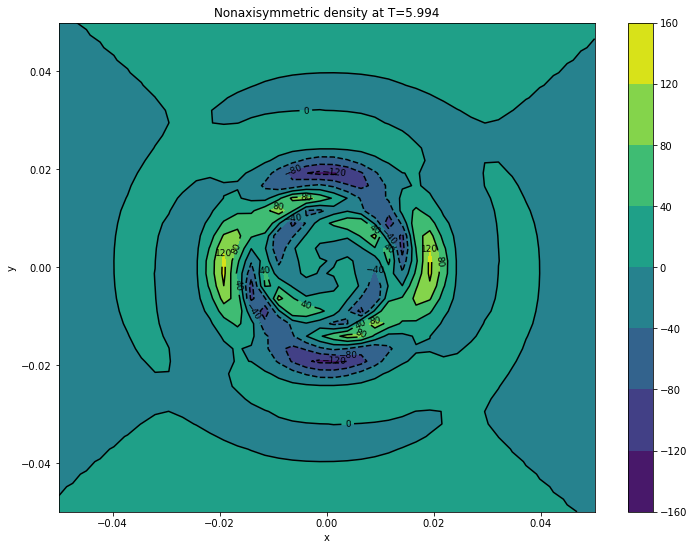
cont1 = plt.contour(xv, yv, surfaces[final]['d1'].transpose(), colors='k')
plt.clabel(cont1, fontsize=9, inline=True)
cont2 = plt.contourf(xv, yv, surfaces[final]['d1'].transpose())
plt.colorbar(cont2)
plt.xlabel('x')
plt.ylabel('y')
plt.title('Nonaxisymmetric density at T={}'.format(final))
plt.show()
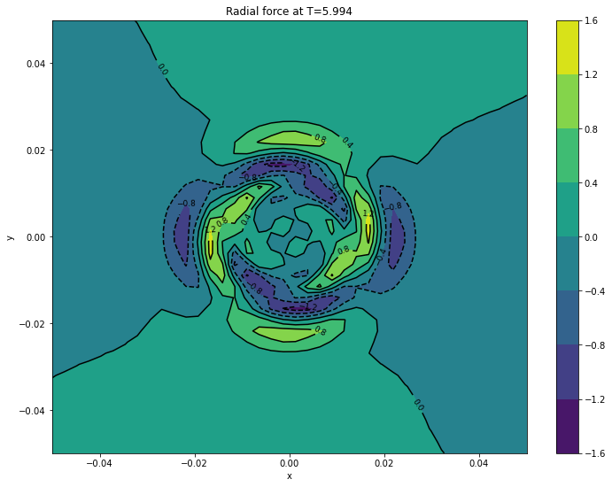
cont1 = plt.contour(xv, yv, surfaces[final]['fr'].transpose(), colors='k')
plt.clabel(cont1, fontsize=9, inline=True)
cont2 = plt.contourf(xv, yv, surfaces[final]['fr'].transpose())
plt.colorbar(cont2)
plt.xlabel('x')
plt.ylabel('y')
plt.title('Radial force at T={}'.format(final))
plt.show()
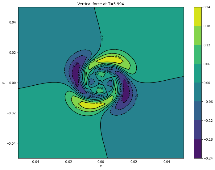
cont1 = plt.contour(xv, yv, surfaces[final]['ft'].transpose(), colors='k')
plt.clabel(cont1, fontsize=9, inline=True)
cont2 = plt.contourf(xv, yv, surfaces[final]['ft'].transpose())
plt.colorbar(cont2)
plt.xlabel('x')
plt.ylabel('y')
plt.title('Vertical force at T={}'.format(final))
plt.show()
The coefficient time list is {} slices in [{}, {}] 1501 0.0 5.998
Creating surfaces with times: [5.994]
Created fields instance
Created surfaces
We now have the following [time field] pairs
----------------------------------------
  5.9940  d
  5.9940  d0
  5.9940  d1
  5.9940  dd
  5.9940  fp
  5.9940  fr
  5.9940  ft
  5.9940  p
  5.9940  p0
  5.9940  p1
Okay, now make a movie
size  = 0.05
npix  = 50
times = coefs.Times()
pmin  = [-size, -size, 0.0]
pmax  = [ size,  size, 0.0]
grid  = [ npix,  npix,   0]

fields = pyEXP.field.FieldGenerator(times, pmin, pmax, grid)

print('Created fields instance')

surfaces = fields.slices(basis[comp], coefs)
# Get the shape
keys = list(surfaces.keys())
nx = surfaces[keys[0]]['d'].shape[0]
ny = surfaces[keys[0]]['d'].shape[1]

# Make the mesh
x = np.linspace(pmin[0], pmax[0], nx)
y = np.linspace(pmin[1], pmax[1], ny)
xv, yv = np.meshgrid(x, y)

plt.rcParams.update({'font.size': 22})

# Fix the contour levels to prevent jitter in the movie (linear scaling)
mval = 200.0
cbar1 = np.arange(-mval, mval, 1.00)
cbar2 = np.arange(-mval, mval, 20.0)

# Frame counter
icnt = 0
cmap = copy.copy(plt.colormaps['viridis'])

N = cmap.N
cmap.set_under(cmap(1))
cmap.set_over(cmap(N-1))

# Iterate through the keys
for v in keys:
    fig, ax = plt.subplots(1, 1, figsize=(24, 20))

    mat = surfaces[v]['d']
    #for i in range(mat.shape[0]):
     #   for j in range(mat.shape[1]):
      #      if mat[i, j] < 1.0: mat[i, j] = 1.0
       #     if mat[i, j] > 10000.0: mat[i, j] = 10000.0

    cont1 = ax.contour(xv, yv, mat.transpose(), cbar2, colors='k')
    # You can label the contours inline by uncommenting the next two lines...
    # ax[0].clabel(cont1, fontsize=9, inline=True)
    # cont2 = ax.contourf(xv, yv, surfaces[v]['d'].transpose(), cbar2, vmin=cbar2[0], vmax=cbar2[-1])
    cont2 = ax.contourf(xv, yv, mat.transpose(), cbar1) #, locator=ticker.LogLocator())
    plt.colorbar(cont2, ax=ax)
    ax.set_xlabel('x')
    ax.set_ylabel('y')
    ax.set_title('T={:4.3f}'.format(v))

    fig.savefig('{}_mssa_{}_{:04d}.png'.format(comp, runtag, icnt), dpi=75)
    plt.close()

    icnt += 1
Make a mp4 file from the frames using ffmpeg
This will only work if you have ‘ffmpeg’ installed, of course …
os.system('ffmpeg -y -i \'{0}_mssa_{1}_%04d.png\' mssa_{0}_{1}.mp4'.format(comp, runtag))